Celestial Labelling
Makoto Takahara / January 2024 (1263 Words, 8 Minutes)
Project Overview
For this project, I classied celestial objects into galaxies, stars, and quasars. This was my submission to DS3 Datathon.
I used machine learning techniques such as decision trees and random forests to make predictions about the class of celestial object given information about telescope angles, various photometric filters, redshift values, and more. This analysis required a blend of knowledge in both statistics and astrophysics, reiterating the importance of domain knowledge in data science.
Project Content
Introduction
This project aims to develop a predictive model for the classification of celestial objects, a critical aspect of astronomical research. Leveraging data from the Sloan Digital Sky Survey, which includes measurements such as telescope angles, photometric filters, and redshift values, we aim to predict whether a celestial object is a star, galaxy, or quasar. Processing this information to make timely decisions is important because asstronomers need to configure their telescopes accordingly before the target objects become unobservable (SDSS).
Multi-label classification tasks are often modelled using decision trees and random forests. Decision trees are statistical models that split data into subsets based on the values of input features, with all data starting at the root of the tree and ending up in a leaf node holding a class label. Random forests are ensemble models containing multiple decision trees that are unique because both observations and factors have been randomly sampled from the full tree. We tailor our methods and models based on our exploratory data analysis to create a predictive model for classifying these celestial objects.
Data
The data was split into training and testing datasets with 50,000 observations each by the Hackathon facilitators. Here is a look at the variables:
id= Object Identifier, the unique value that identifies the object in the image catalog used by the CAS.alpha= Right Ascension angle (at J2000 epoch).delta= Declination angle (at J2000 epoch).u= Ultraviolet filter in the photometric system.g= Green filter in the photometric system.r= Red filter in the photometric system.i= Near Infrared filter in the photometric system.z= Infrared filter in the photometric system.run_ID= Run Number used to identify the specific scan.rerun_ID= Rerun Number to specify how the image was processed.cam_col= Camera column to identify the scanline within the run.field_ID= Field number to identify each field.spec_obj_ID= Unique ID used for optical spectroscopic objects (this means that 2 different observations with the same spec_obj_ID must share the output class).redshift= redshift value based on the increase in wavelength.plate= plate ID, identifies each plate in SDSS.MJD= Modified Julian Date, used to indicate when a given piece of SDSS data was taken.fiber_ID= fiber ID that identifies the fiber that pointed the light at the focal plane in each observation.class= object class [GALAXY: galaxy, STAR: star or QSO: quasar object].
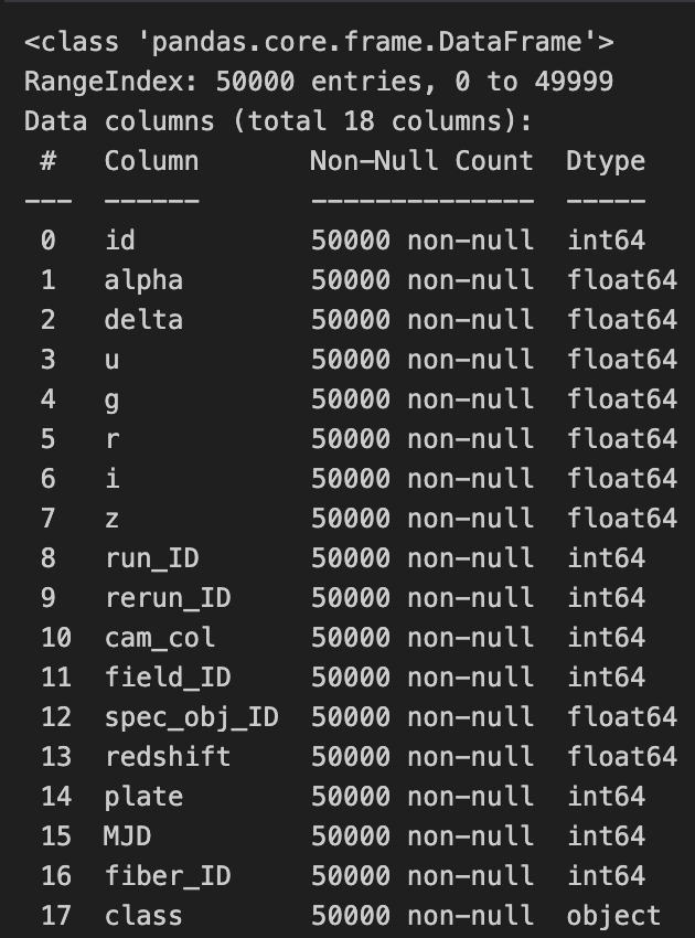
All variables are currently numeric. However, some are not appropriate for predictive modelling as it is. For example, all of the variables with names ending in ID are categorical, using numbers as labels for each category. After research into the meaning of each variable, we convert id, run_ID, rerun_ID,cam_col, field_ID, spec_obj_ID, fiber_ID, plate, MJD to categocial variables.
Next, we explore the numerical variables.
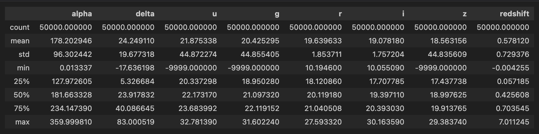
We see that the minimum of u, g, z is -9999.000000, which we would not expect in this context. Flux values represent the amount of light detected from a celestial object in a specific wavelength range, and negative flux values would not have a physical interpretation in this context (CITE). We find that it is the same observation with these values, so we remove this observation from the training dataset. Also, rerun_ID is the same for all the observations. Thus, we disregard this variable from here onwards.
Exploratory Data Analysis
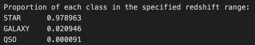
We plot a kernel density estimate Plot to summarize the distribution of the numerical variables for each class of celestial object.
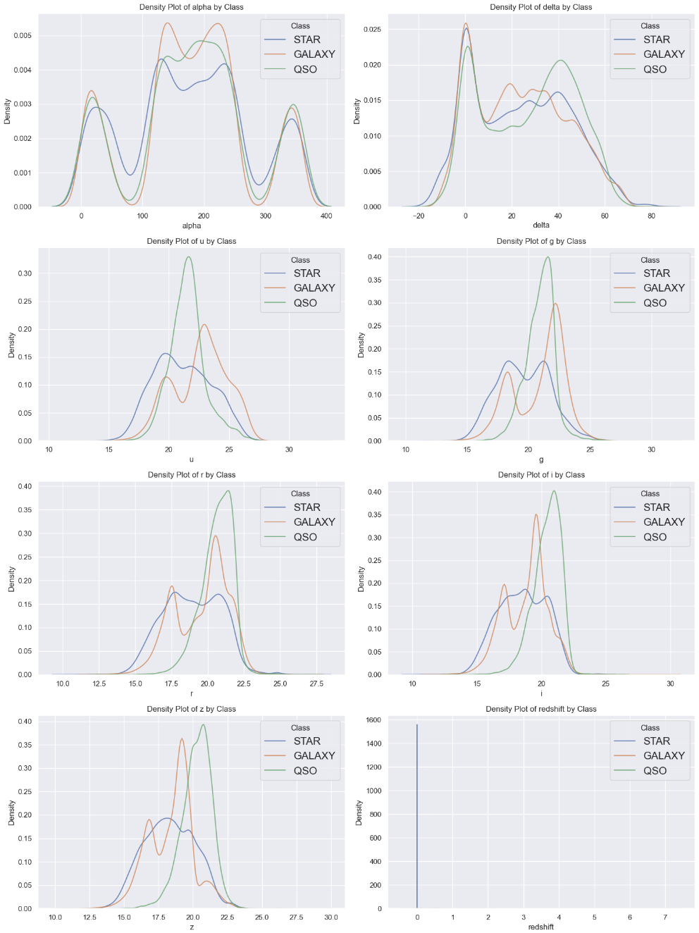
For all of the variables except for redshift, we can observe varying distributions for each class. The KDE plot for redshift looks pelicular, and we dig deeper to find that all 10703 observations of the star class has redshift between -0.0042 and 0.0042. We also find that within this range, 97.9% of observations are of the star class.
We also perform a Chi-squared test to determine if there is a statistically significant relationship between each categorical variable and the respone variable class.
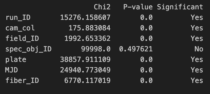
We see that spec_obj_ID does not have a statistically significant relationship with the predictor variable. With this information in mind, we move onto fitting some predictive models.
Decision Tree
Firstly, we are certain that if different observations have the same spec_obj_ID, it will be of the same class. Therefore, before fitting any predictive model, we map spec_obj_ID to class using a dictionary. Then, we apply this mapping to the testing data to make classifications. For the observations in the testing data that have not been classified after this process, we predict its class using a decision tree.
We fit the decision tree on the training dataset with the all variables except for rerun_ID and spec_obj_ID, which we determined to be irrelevant with respect to our predictive model. A decision tree is a statistical model that splits data into subsets based on the values of input features. All data starts at the root of the tree and ends up in a leaf node holding a class label.
We then use this model to make predictions on the testing dataset. Finally, we merge the predictions of the decision tree with the mapping prediction. The accuracy of our predictions on the testing dataset was: 0.9597834.
Random Forest
A random forest is a statistical method that constructs multiple decision trees and aggregates their results. Each tree is built from a random subset of data and random subset of features, leading to a forest of diverse trees that together yield a more robust prediction.
We again check if any testing data can be mapped from spec_obj_ID to class using a dictionary. Then, we fit a random forest with the same variables. The proportion of observations classified as star for the specified redshift range -0.0042 and 0.0042 is 99.22%, in line with our expectations from the exploratory data analysis. This intuition is support by an accuracy of 0.97133065 on the testing data, an improvement over the decision tree.
We perform a feature importance analysis with a table of importances and a plot of cumulative importance. This helps ensure that we do not overfit our model to the training data.
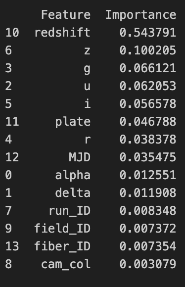
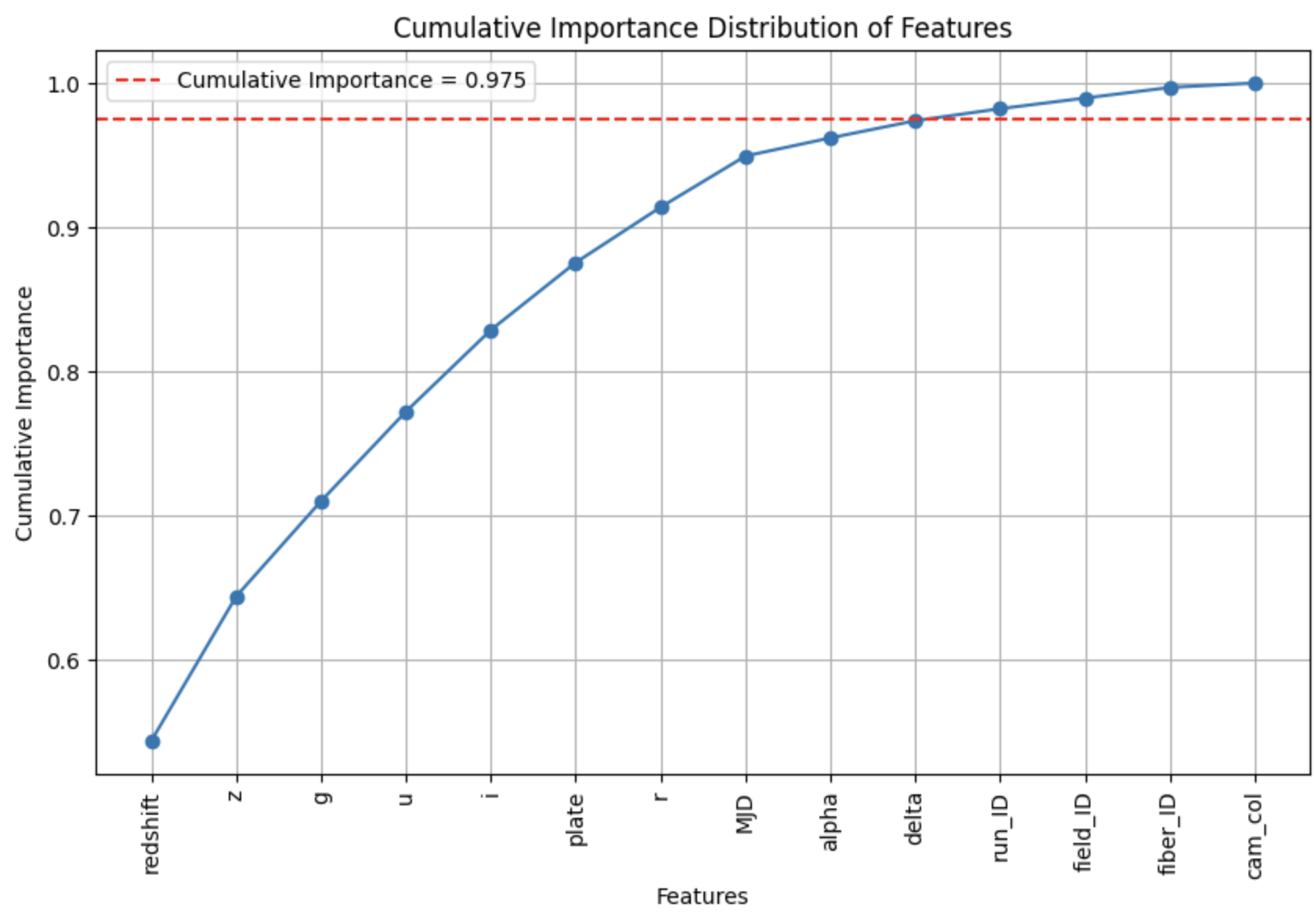
Though our threshold of 0.975 is arbitrary, we remove run_ID, field_ID, fiber_ID, and cam_col as they are the relatively insignificant factors according to our classification. We fit another random forest. Our accuracy on the testing data improves again to 0.97235535.
Conclusion
We used a random forest with redshift, z, i, g, u, plate, ‘r’, MJD, alpha, delta to attain an accuracy of 0.97235535 on the testing data when classifying celestial objects as stars, galaxies, or quasars. Knowledge in both statistics and astrophysics throughout the analysis process, from adjusting variable types and identifying outliers to fitting the model and selecting factors.
Some limitations of this classification include potential overfitting, inability to handle new types of celestial objects not present in the training data, and the reliance on the quality and completeness of the Sloan Digital Sky Survey data.
In future studies, it would be beneficial to incorporate additional data sources, try different machine learning models, and apply techniques to handle class imbalance.
References
- Trott, T. (2023). Brightness, Luminosity and Flux of Stars Explained. Perfect Astronomy. Link
- Sloan Digital Sky Survey. (n.d.). Data. SkyServer. Link