Election Prediction
Makoto Takahara / January 2024 (3744 Words, 21 Minutes)
Project Overview
For this project, I worked in a group to predict the proportion of votes each party will recieve in the 2025 Canadian Federal Election.
We used multilevel regression with poststratification with data from the General Social Survey (GSS), a comprehensive national survey by Statistics Canada, and the 2021 Canadian Election Study (CES), a specialized study focusing on Canadian federal elections. This project placed an emphasis on considering both individual-level and group-level variations in hierarchical data and adjusting for population characteristics through post-stratification.
Project Content
Introduction
As the 2025 Canadian federal election approaches, we aim to predict the party that will secure the highest proportion of the popular vote. This prediction is crucial for anticipating potential policy changes and shifts in government priorities.
However, accurately representing the diverse political preferences of Canadians is challenging due to potential biases in survey data, such as non-response bias, social desirability bias, and sampling bias. To address these, we use a multilevel regression model with post-stratification (MRP), combining demographic data from the General Social Survey (GSS) and survey data from the 2021 Canadian Election Study (CES). By utilizing both datasets, MRP can address some of the challenges by using detailed demographic information from sources like the General Social Survey (GSS) to make the survey data more representative and precise. It helps compensate for non-response bias, sampling bias, and other biases by incorporating additional information to create more accurate predictions, ensuring that the survey results better reflect the diverse opinions of the Canadian population (Holt & Smith, 1979).
We hypothesize that the incumbent Liberal Party is more likely to secure victory in the next Canadian federal election in 2025. This hypothesis is based on historical patterns of incumbents often benefiting from the advantages of name recognition, established infrastructure, and the ability to campaign on their record of governance (Lucas et al., 2021). Additionally, the Liberal Party’s historical performance and policy positions may position them favorably with the electorate.
Data
Datasets
The General Social Survey (GSS) in 2016 used a two-stage sampling design to collect data from households across Canada. The sampling units were groups of telephone numbers, and the final stage units were individuals within the identified households. The survey employed a stratified sampling method, dividing the ten provinces into 27 strata based on geographic areas, including Census Metropolitan Areas (CMAs) and non-CMA regions. Minimum sample sizes were determined for each stratum to ensure acceptable sampling variability, and the remaining sample was allocated to balance the precision of national and stratum-level estimates. The GSS randomly selected one eligible member aged 15 or older from each sampled household to complete the questionnaire. Approximately 43,000 units were included in the field sample, with around 35,000 invitation letters sent to selected households, and an expected completion of 20,000 questionnaires. Data collection was voluntary and direct from survey respondents (Statistics Canada, n.d.).
The Canadian Election Study (CES) data collection process for the 2021 election involved a two-wave panel. The Campaign Period Survey (CPS) gathered a sample of 20,968 members of the Canadian population through the Leger Opinion panel, stratified by region and balanced for gender and age within each region. The CPS consisted of three waves, collecting data from August to September 2021. After the election, 15,069 respondents completed the Post-Election Survey (PES) from late September to early October 2021, resulting in a return rate of 72%. Data quality checks were applied to remove incomplete, duplicate, or low-quality responses (Stephenson et al., 2022).
Data Cleaning
Census Dataset
-
Selecting columns that will be used for the model
We selected specific variables (columns) that will be included in the model. Specifically, the selected variables are ‘age’, ‘marital_status’, ‘citizenship_status’, ‘province’, ‘education’, and ‘pop_center’. These variables are selected based on a study from Statistics Canada which shows significant variables in determining voter decisions. It shows marginal effects from a probit model of voting, which provides insights into how changes in the independent variables affect the probability of an individual voting in a particular election or engaging in a binary outcome, such as “voting” or “not voting.” (Statistics Canada, 2015) -
Mutating the categorical column so that each column has a numerical value
A new variable ‘marital’ is created, representing marital status. It is recoded based on the ‘marital_status’ variable. The recoding assigns numerical values 1 to 7 for various marital status categories, with 1 representing “Married,” 2 for “Living common-law,” 3 for “Divorced,” 4 for “Separated,” 5 for “Widowed,” 6 for “Single, never married,” and 7 for any other status. A new variable ‘bornin_canada’ is created to represent citizenship status. It is recoded based on the ‘citizenship_status’ variable, with 1 for “By birth,” 2 for “By naturalization,” and 3 for “Don’t know.”
A new variable ‘province’ is created to represent the province of residence. It is recoded based on the ‘province’ variable. Each province is assigned a unique numeric value from 1 to 13, with 1 representing “Alberta,” 2 for “British Columnia,” 3 for “Manitoba,” 4 for “New Brunswick,” 5 for “Newfoundland and Labrador,” 6 for “Northwest Territories,” 7 for “Nova Scotia,” 8 for “Nunavut,” 9 for “Ontario,” 10 for “Prince Edward Island,” 11 for “Quebec,” 12 for “Saskatchewan,” 13 for “Yukon.”
A new variable ‘education’ is created to represent the level of education. It is recoded based on the ‘education’ variable. Numeric values are assigned to different education categories, with 5 for “High school diploma,” 7 for “Trade certificate or diploma” and “College, CEGEP or other non-university certificate or diploma,” 9 for “Bachelor’s degree (e.g. B.A., B.Sc., LL.B.),” 4 for “Less than high school diploma or its equivalent,” 8 for “University certificate or diploma below the bachelor’s level,” 9 for “University certificate, diploma or degree above the bachelor’s level,” and NA (representing missing values) if none of the above conditions are met.
A new variable ‘rural_urban’ is created to represent the population center. It is recoded based on the ‘pop_center’ variable. Values 5 and 3 are assigned to “Larger urban population centres’’ and “Rural areas and small population centres,” respectively. Other values are set as missing (NA). -
Variable Rounding
The ‘age’ column is rounded to the whole number for consistency with the Campaign Period Survey. -
Column Removal
Columns ‘marital_status’, ‘citizenship_status’, ‘province’, ‘education’, ‘pop_center’, and ‘age’ are removed from the dataset as they are no longer needed. -
Filtering
Rows in which the ‘age’ variable is less than 18 are filtered out because the model is trained on individuals aged 18 and above. -
Removing Missing Values
Any rows with missing values (NA) are dropped from the dataset.
Survey dataset:
- Variable Selection
We selected specific columns in the survey_data dataset for inclusion in the model_data dataset. These selected columns are:
- ‘cps21_votechoice’: Represents the respondent’s vote choice.
- ‘cps21_age’: Represents the respondent’s age.
- ‘cps21_marital’: Represents the respondent’s marital status.
- ‘cps21_bornin_canada’: Represents the respondent’s citizenship status (whether born in Canada or not).
- ‘cps21_province’: Represents the respondent’s province of residence.
- ‘cps21_education’: Represents the respondent’s level of education.
- ‘pes21_rural_urban’: Represents the respondent’s area of residence, indicating whether it is within a population center and its urban/rural designation. Similar to the census dataset, the selection is based on the study from Statistics Canada which shows significant variables in determining voter decisions (Statistics Canada, 2015).
- Removing Missing Values
The drop_na() function is used to remove rows with missing values from the model_data dataset. This step ensures that only complete cases with data in all selected columns are retained in the final dataset.
The result is a cleaned and filtered dataset named model_data that includes the specified variables for further analysis. Then, for census data, we cleaned it so that it matches the inputs as the survey data.
Description of the important variables
- Vote choice (cps21_votechoice): Represents the respondent’s vote choice.
- Age (age & cps21_age): Represents the age of respondents. It is rounded in the cleaning process.
- Marital status (marital & cps21_marital): Represents the marital status of respondents. 1: “Married” 2: “Living common-law” 3: “Divorced” 4: “Separated” 5: “Widowed” 6: “Single, never married” 7: For any other or unexpected values in ‘marital_status’.
- Citizenship status (bornin_canada & cps21_bornin_canada): Represents the citizenship status of respondents. 1: “By birth” 2: “By naturalization” 3: “Don’t know” (If this category is present in the original data).
- province & cps21_province: Represents the province of residence. Numeric codes from 1 to 13 for different provinces and territories.
- Education (education & cps21_education): Represents the level of education of respondents. 4: “Less than high school diploma or its equivalent” 5: “High school diploma or a high school equivalency certificate” 7: “Trade certificate or diploma” or “College, CEGEP or other non-university certificate or diploma” 8: “University certificate or diploma below the bachelor’s level” 9: “Bachelor’s degree (e.g. B.A., B.Sc., LL.B.)” and 11: “University certificate, diploma or degree above the bachelor’s level” NA: For any other or unexpected values in ‘education’.
- Town size (rural_urban & pes21_rural_urban): Represents the respondent’s location in terms of population center and urban/rural designation, providing information about the urban or rural nature of their residence. 3: “Rural areas and small population centres (non CMA/CA)” 5: “Larger urban population centres (CMA/CA)” NA: For any other or unexpected values in ‘pop_center’.
Table 1: Summary Statistics for Census and Survey Datasets
| Census Data | Survey Data | |
|---|---|---|
| Survey Size | 18210 | 10498 |
| Mean Age | 53 | 53 |
| Standard Deviation of Age | 17.088% | 16.616% |
| Percentage of Individuals Born in Canada | 83.992% | 85.311% |
| Percentage of Individuals living in Larger Urban Population Centres | 79.412% | 69.575% |
From the summary statistics in Table 1, the census data has more data points than the survey dataset after dropping for missing values. For mean and standard deviation of age, the census and survey datasets have similar numerical results. The percentage of individuals born in Canada is similar between the two as well. These values suggest that the CES survey dataset is representative of the population.
However, the proportion of respondents from “Larger urban population centres” is approximately 10 percentage points higher in census data than survey data. Factors such as varying survey participation rates, engagement with online surveys, and regional differences in civic involvement might contribute to this divergence in representation. Recognizing that these discrepancies may introduce bias, we use post-stratification in our analysis.
Next, we examine data for the categorical variables with multiple levels through bar plots.
Figure 1 represents a bar plot comparing the distribution of respondents’ provinces in census and survey data. To streamline visualization, provinces excluding Ontario, Quebec, Alberta, and British Columbia were grouped in an “others” category. The observed higher frequency for Ontario and Quebec in the survey data, compared to the greater frequency of grouped “other” provinces in the census data, could result from grouping considerations and regional differences in survey response rates. Variations in response motivations influenced by cultural, socio-economic, or regional factors may contribute to observed discrepancies.
Figure 1: Bar plot of Province of Residence
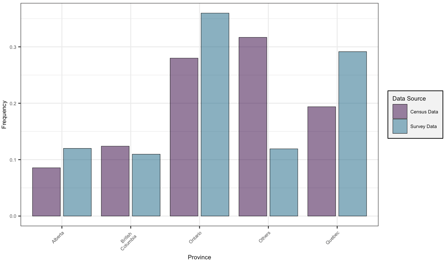
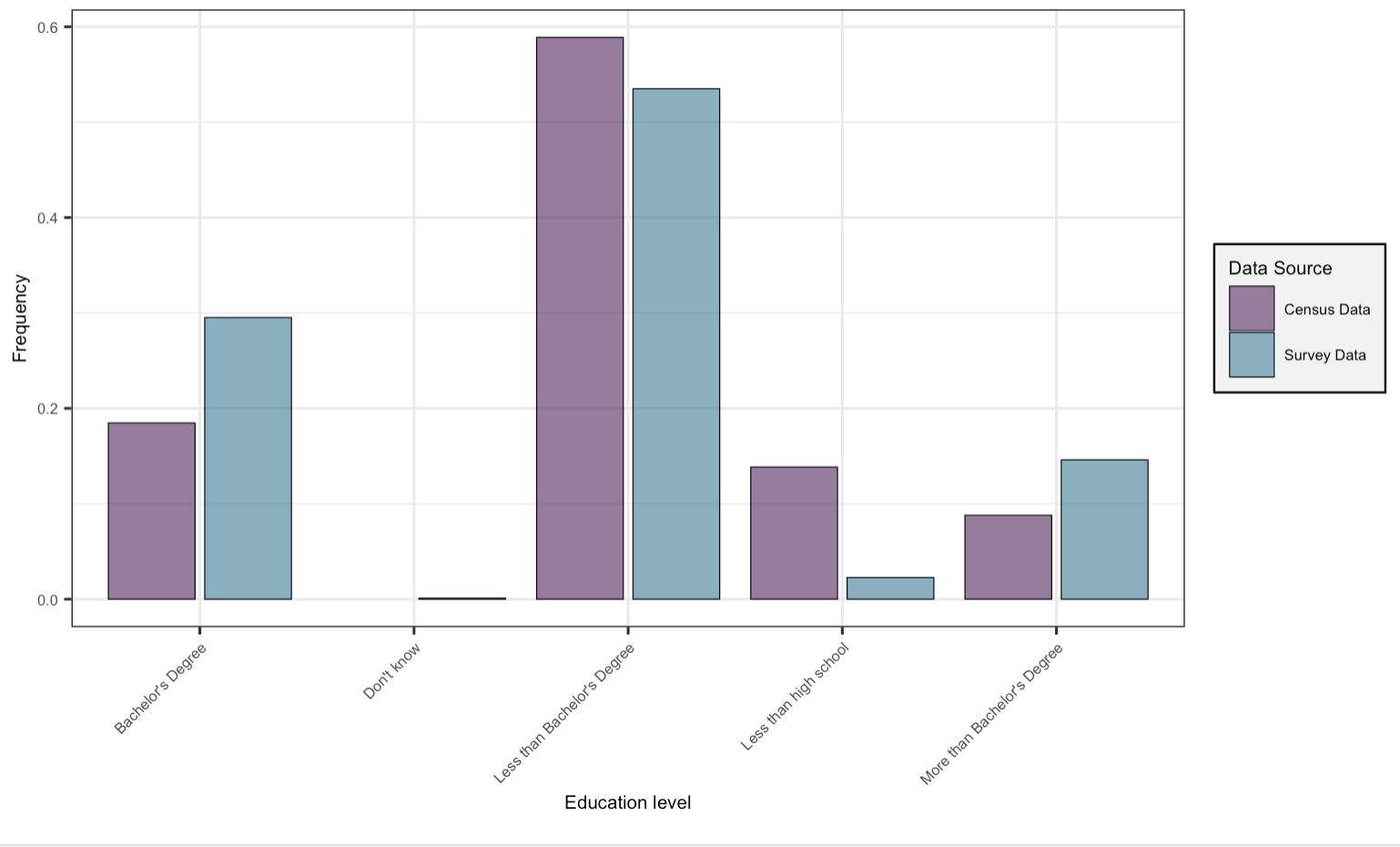
Figure 2 depicts a histogram comparing the distribution of respondents’ education levels between census and survey data. To enhance visual clarity, categories in both datasets were consolidated into “Less than high school,” “Less than Bachelor’s Degree,” “Bachelor’s Degree,” “More than Bachelor’s Degree,” and “Don’t know.” The figure indicates a higher prevalence of respondents with completed “Bachelor’s Degree” and “More than Bachelor’s Degree” in the survey data compared to the census data. Conversely, there is a greater representation of respondents who completed “Less than high school” and “Less than Bachelor’s Degree” in the census data relative to the survey data. This observed difference suggests that survey respondents tend to have slightly higher education levels than individuals in the census. Possible explanations for this discrepancy may stem from the likelihood that well-educated individuals approach the election survey with greater seriousness compared to those with lower levels of education.
These two visualizations motivate the use of post-stratification in our analysis, ensuring a more accurate representation of the overall population and addressing biases introduced during data collection.
Figure 2: Bar plot of Educational Attainment
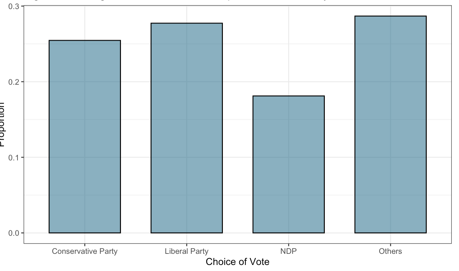
Finally, Figure 3 shows the raw proprtion of vote choice for each party. Given the differences between the census data and the survey data, these raw proportions may not be representative of the actual election results.
Figure 3: Bar plot of Vote Choice
Methods
The goal of this study is to predict the party winning the popular vote in the upcoming Canadian Federal Election. Thus, our parameter of interest is the percentage of the popular vote that each party will receive in the upcoming elections, from which we can deduce the party that wins the election. We will use a multilevel regression and poststratification to estimate this parameter of interest. This approach involves partitioning the data into many demographic cells, estimating the preferred party in each cell with a statistical model, then aggregating each of the responses by weighting each cell by its proportion to the population.
Model Specifics
Firstly, we fit a statistical model that will be used to make predictions in each demographic cell. We selected a multinomial logistic regression due to the nature of our outcome variable, party of choice, as there are multiple possible discrete outcomes. This approach enables us to effectively model the influence of various factors on the voting preferences within each demographic category.
While there are a multitude of factors that may influence a demographic to vote for a certain party, we make the decision to include age, marital status, Canadian or foreign born, province of residence, education, and living in rural or urban areas as factors including this choice in our model. We fit this using the election data, as we have information about all of these factors as well as the parties that these individuals are looking to vote for. Our model is:
\[\begin{align} \log\left(\frac{P(Y = j)}{P(Y = K)}\right) & = \beta_{0j} + \beta_{1j}x_{\text{age}} + \beta_{2j}x_{\text{marital status}} + \beta_{3j}x_{\text{canadian or foreign born}} \nonumber\\ & \quad + \beta_{4j}x_{\text{province of residence}} + \beta_{5j}x_{\text{education}} + \beta_{6j}x_{\text{living in rural or urban areas}} + \epsilon_j, \nonumber \end{align}\]Where $j$ is a nominal variable arbitrarily assigned to each party and $k$ is the a baseline party, which is also arbitrarily chosen as a reference. $\beta_{0j}$ is the intercept for the jth party, so $\beta_{01}$ would be the intercept for the party assigned the nominal value 1. Similarly, the following coefficients represent how much the presence of that factor is associated with a change in the log odds of the ratio between the party in question and the baseline party.
This combination of factors is justified through our analysis using the Akaike Information Criterion, which allows us to estimate the quality of a model compared to others. Out of all possible permutations of these factors, we obtained the best result using all of them. Thus, it is necessary for us to remove all observations where data is missing - we need all of this data for the highest quality model.
Poststratification
This is followed by a process called poststratification, in which we can use the fitted model to predict how certain a demographic group will vote. Then, we can weight the outcomes from each demographic group based on how common we expect these demographic groups to exist in the population, with the final sum allowing us to make predictions about the popular vote. The poststratification estimates of an sample proportion are defined by the following equations:
$$\hat{y}^{PS}_{\text{liberal}} = \frac{\sum_{j=1}^{J}N_j\hat{y}_{j\text{liberal}}}{\sum_{j=1}^{J}N_j}$$
$$\hat{y}^{PS}_{\text{conservative}} = \frac{\sum_{j=1}^{J}N_j\hat{y}_{j\text{conservative}}}{\sum_{j=1}^{J}N_j}$$
$$\hat{y}^{PS}_{\text{ndp}} = \frac{\sum_{j=1}^{J}N_j\hat{y}_{j\text{ndp}}}{\sum_{j=1}^{J}N_j}$$
$$\hat{y}^{PS}_{\text{bloc}} = \frac{\sum_{j=1}^{J}N_j\hat{y}_{j\text{bloc}}}{\sum_{j=1}^{J}N_j}$$
$$\hat{y}^{PS}_{\text{other}} = \frac{\sum_{j=1}^{J}N_j\hat{y}_{j\text{other}}}{\sum_{j=1}^{J}N_j}$$
For this step, we move from the election data to the census data. This data has information about all of the factors we included in the model (age, marital status, etc), but does not contain data about electoral preferences. After grouping individuals with the same characteristics, we use the fitted model to predict the party that this demographic group would vote for. The party with the highest log odds is noted as a party of choice for that demographic group. Finally, we aggregate these results, weighted by the size of the group with these characteristics. This allows us to predict the popular vote.
Results
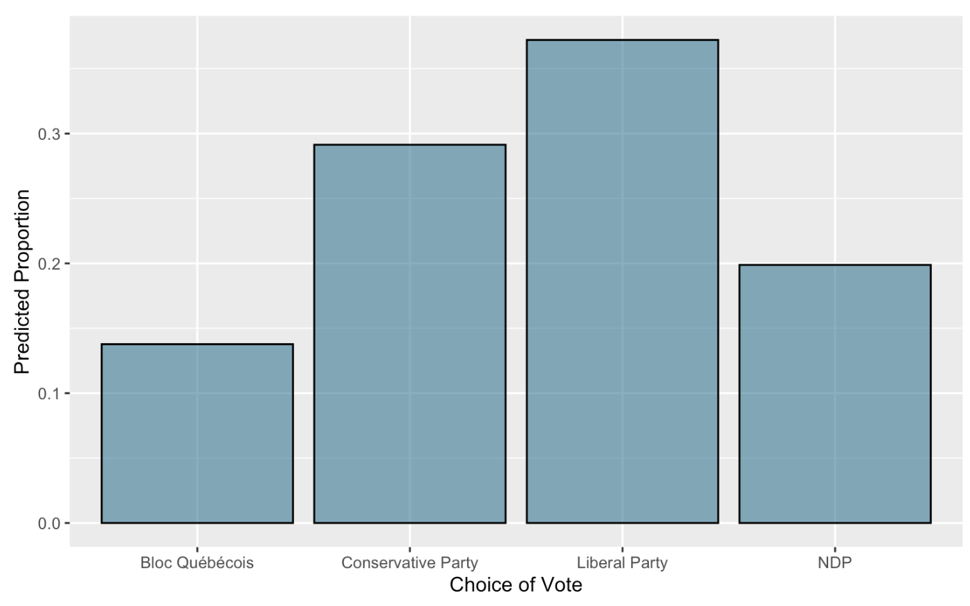
The results of our study are summarized in Table 2 and Figure 4.
Our model predicts that the Liberal Party will win with 37.2% of the popular vote. The Conservative Party comes second with 29.1%, while the NDP gets 19.9% of the vote to place third. The model predicts Bloc Québécois coming fourth with 13.8% of the vote. Finally, the model predicts that all other parties including the Green Party will get 0% of the popular vote.
To determine if the model’s predictions are reasonable, we compare these values to the actual results of the 2021 Canadian Federal Election. In 2021, the Liberal Party had 32.6% of the vote. The Conservative Party had 33.7%, while the NDP had 17.8%. Bloc Québécois had 7.6% and the Green Party had 2.3%. Other parties had a total of 5.9% (CBC/Radio Canada, n.d.).
While factors such as a changing political landscape or difference in campaign dynamics prevent the 2021 election results from being a perfect reference for future outcomes, we can still gain insights from these past results. The 2021 Canadian Federal Election, broadly speaking, has a similar proportion of voters for each party. This is as expected as it has only been 2 years since the previous election, so we do not expect a drastic change in voter preference. Thus, it suggests that the results of our study are reasonable estimates for the proportion of the popular vote that each party will receive.
These results help us answer the research question of who will have the highest proportion of the popular vote win the 2025 elections. Our final prediction is that the Liberal Party will in the popular vote.
Table 2: Predicted Popular Vote by Party |Party| Popular Vote| |:-:|:-:| | Liberal Party |37.2%| | Conservative Party |29.1%| | NDP |19.9%| | Bloc Québécois |13.8%| | Green |0%| | Other |0%|
Figure 4: Predicted Popular Vote by Party
Conclusion
We set out to predict the result of the 2025 Canadian Federal Election using data. Our starting idea was that the current ruling Liberal Party might win again, considering past trends. Our method employed a sophisticated multilevel regression and poststratification model called multinomial logistic regression, based on detailed demographic data from the General Social Survey and survey data from the 2021 Canadian Election Study. We tried to make sure our predictions representitive of the voting population by dealing with problems like some people not wanting to answer our questions and making sure our surveyed group looked like the whole population.
Our model anticipates the Liberal Party securing victory with 37.2% of the popular vote, followed by the Conservative Party at 29.1%, and the NDP at 19.9%. The Bloc Québécois is expected to secure 13.8% of the vote, while all other parties, including the Green Party, are predicted to receive 0%.
To validate the model’s predictions, we compared them with the 2021 Canadian Federal Election results (CBC/Radio Canada, n.d.). While acknowledging the potential for changes in the political landscape, the close alignment of our predictions with the 2021 outcomes suggests that our estimates for the proportion of the popular vote are reasonable. The findings suggest that the same pattern of proportional distribution seen in the last election is likely to persist, supporting the idea that the Liberal Party is expected to win again in 2025.
Our model’s prediction of the Liberal Party’s success can be attributed to historical advantages associated with incumbency, such as name recognition, established infrastructure, and the ability to campaign on a record of governance (Lucas et al., 2021). The factors influencing voter preferences, including age, marital status, place of residence, education, and urban or rural living, were carefully considered in the model, providing a understanding of the electorate.
One drawback of this study is that the popular vote may not be representative of the influence that a party has on the Canadian government. The discrepancy between popular vote and the proportion of seats won in the House of Commons is a noted feature of Canada’s “First Past the Post” voting system (Ansolabehere & Leblanc, 2008). This means that even though we predict the Liberal Party to have the largest support in terms of the popular vote, this model does not help predict the party with the most seats in the House of Commons and the most influence on Canadian policy. Additionally, reliance on historical patterns assumes that voter behavior is stable, which may not fully capture evolving societal trends or unforeseen events that could influence the election.
For future analyses or reports, it is crucial to continuously update and refine our model as new data becomes available. Ongoing monitoring of political developments, public sentiment, and emerging issues should inform adjustments to the model parameters. Incorporating real-time data and adapting to evolving trends will enhance the predictive accuracy of our approach. Additionally, exploring the impact of external factors, such as global events or economic shifts, could further enrich the depth of our predictions. Also, we would like to perform an analysis that is more consistent with the Canadian electoral system in future studies.
In conclusion, our data-driven exploration illuminates a probable outcome for the 2025 Canadian Federal Election, with the Liberal Party expected to lead the popular vote. While there’s always some uncertainty, this analysis gives useful insights for planning and decision-making in the upcoming political scene.
References
-
Allaire, J.J., et al. (n.d.). Introduction to R Markdown. RStudio. Link. (Last Accessed: November 16, 2023)
-
Ansolabehere, S., & Leblanc, W. (2008). A spatial model of the relationship between seats and votes. Mathematical and Computer Modelling, 48(9–10), 1409–1420. DOI
-
CBC/Radio Canada. (n.d.). Federal election 2021 live results. CBCnews. Link
-
Grolemund, G. (2014, July 16). Introduction to R Markdown. RStudio. Link. (Last Accessed: November 16, 2023)
-
Holt, D., & Smith, T. M. (1979). Post stratification. Journal of the Royal Statistical Society. Series A (General), 142(1), 33. DOI
-
Lucas, J., McGregor, R. M., & Tuxhorn, K.-L. (2021). Closest to the people? Incumbency advantage and the personal vote in non-partisan elections. Political Research Quarterly, 75(1), 188–202. DOI
-
Mayer, A. (2021). Reducing respondents’ perceptions of bias in survey research. Methodological Innovations, 14(3), 205979912110559. DOI
-
Northcott, R. (2015). Opinion polling and election predictions. Philosophy of Science, 82(5), 1260–1271. DOI
-
RStudio Team. (2020). RStudio: Integrated Development for R. RStudio, PBC, Boston, MA. Link.
-
Statistics Canada. (2015, November 27). Labour Force Survey, May 2011. Link
-
Statistics Canada. (n.d.). General Social Survey: Canadians at Work and Home (GSS). Link
-
Stephenson, L. B., Harell, A., Rubenson, D., & Loewen, P. J. (2022). 2021 Canadian Election Study (CES) [Data set]. Harvard Dataverse. DOI