Heart Disease Classification
Makoto Takahara / January 2024 (1622 Words, 10 Minutes)
Project Overview
For this project, I predicted whether a presence of heart disease in patients.
I used classification using logistic regression based on information such as a patient’s age, sex, cholesterol levels, and resting blood pressure.
Project Content
Introduction
This project aims to develop a predictive model for detecting the presence of heart disease, utilizing key factors such as age, maximum heart rate, and cholesterol levels. Beyond its significance in advancing public health and cardiovascular research, the impact of detecting heart disease extends to individuals’ well-being on a micro level. Our exploration of various factors relies on data from the UCI Heart Disease Dataset, with the goal of developing a robust model for this purpose.
Logistic regression, a foundational statistical method in binary classification, plays a pivotal role in this project. By fitting a sigmoid function to the data, it transforms a combination of features into a probability scale ranging from 0 to 1. Typically, a threshold of 0.5 is set to predict whether an observation indicates the presence (1) or absence (0) of heart disease. The relative simplicity and interpretability of logistic regression make it a powerful and reliable tool for binary classification tasks.
Data
The data was split into training and testing datasets with 643 and 275 observations respectively by the Hackathon facilitators. Here is a look at the variables:
Age: age of the patient [years]Sex: sex of the patient [M: Male, F: Female]ChestPainType: chest pain type [TA: Typical Angina, ATA: Atypical Angina, NAP: Non-Anginal Pain, ASY: Asymptomatic]RestingBP: resting blood pressure [mm Hg]Cholesterol: serum cholesterol [mm/dl]FastingBS: fasting blood sugar [1: if FastingBS > 120 mg/dl, 0: otherwise]RestingECG: resting electrocardiogram results [Normal: Normal, ST: having ST-T wave abnormality (T wave inversions and/or ST elevation or depression of > 0.05 mV), LVH: showing probable or definite left ventricular hypertrophy by Estes’ criteria]MaxHR: maximum heart rate achieved [Numeric value between 60 and 202]ExerciseAngina: exercise-induced angina [Y: Yes, N: No]Oldpeak: oldpeak = ST [Numeric value measured in depression]ST_Slope: the slope of the peak exercise ST segment [Up: upsloping, Flat: flat, Down: downsloping]HeartDisease: output class [1: heart disease, 0: Normal]
From this, we observe that there is a undocumented Unnamed: 0 variable that contains 0 in all observations. We disregard this variable in our analysis.
Exploratory Data Analysis
Univariate Analysis
First, we explore the distribution of numerical variables.
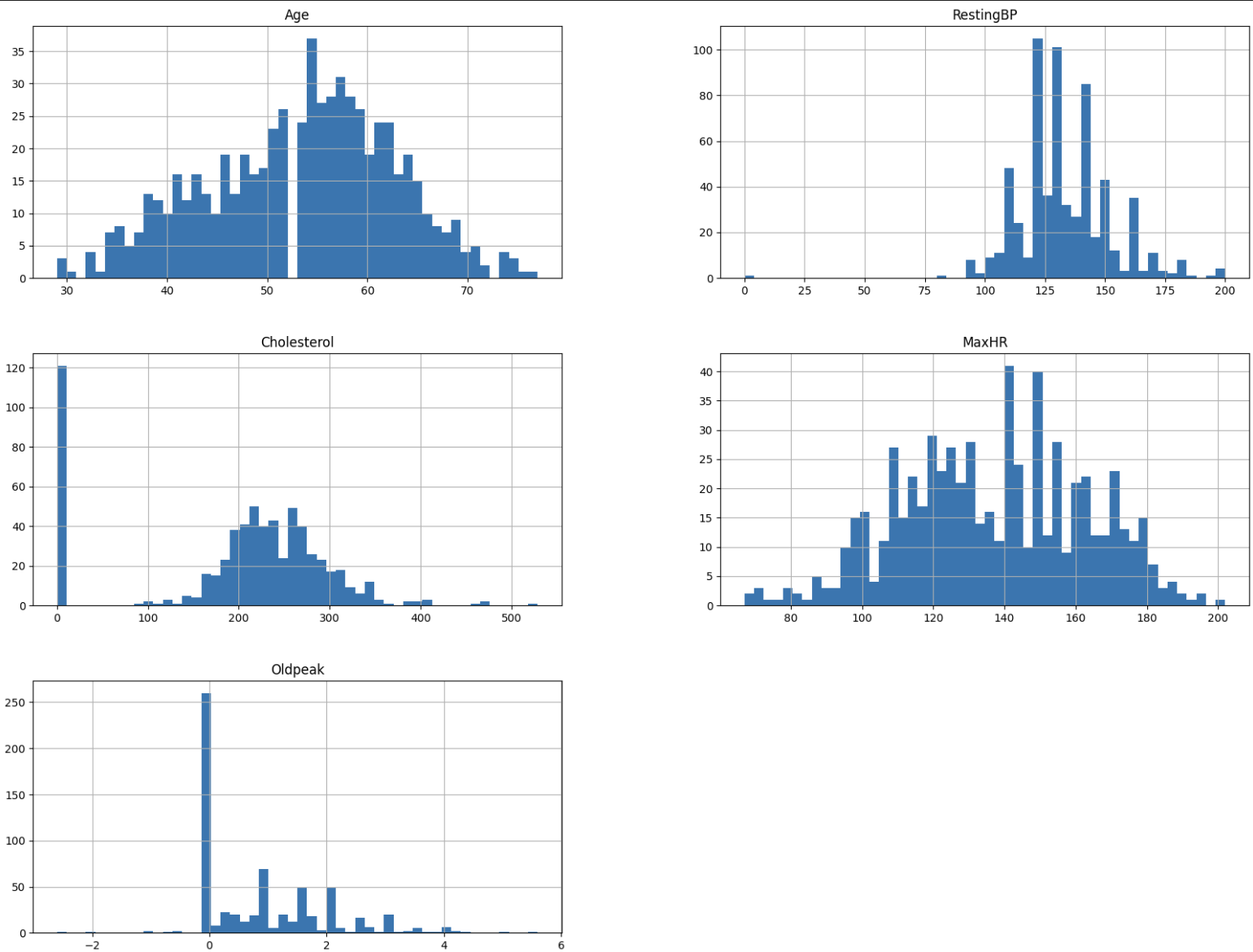
Upon visual inspection, there seem to be odd characteristics in some of the variables. For example, there is an empty bin in Age at 53. We also obvseve possibly unnatural peaks at 0 in Cholesterol and Oldpeak. 0 for Oldpeak seems to be plausible given that it is a value relative to RestingECG. On the other hand, we found that 0 mg/dl of cholesterol is not within a realistic range, as values below 70 mg/dl are reported as “abnormally low” even under the secondary prevention settings (Tada et al., 2020). We suspect that there may have been measurement error or missing values.
However, given that 121 out of 643 observations in the training dataset has 0 for Cholesterol, it is difficult to remove these observations altogether. Furthermore, the testing dataset also contains a high proportion of observations with 0 for Cholesterol, so we note this abnormality as we go forward with our analysis.
We also observe some outliers from these histograms, so we will identify them using z-scores with a threshold of 3. We have 13 outliers, which we will remove from the analysis. Before removal, our training dataset had 643 observations. After the removal of 13 outliers, we now have 630 observations in our dataset.
Next, we explore the distribution of categorical variables.
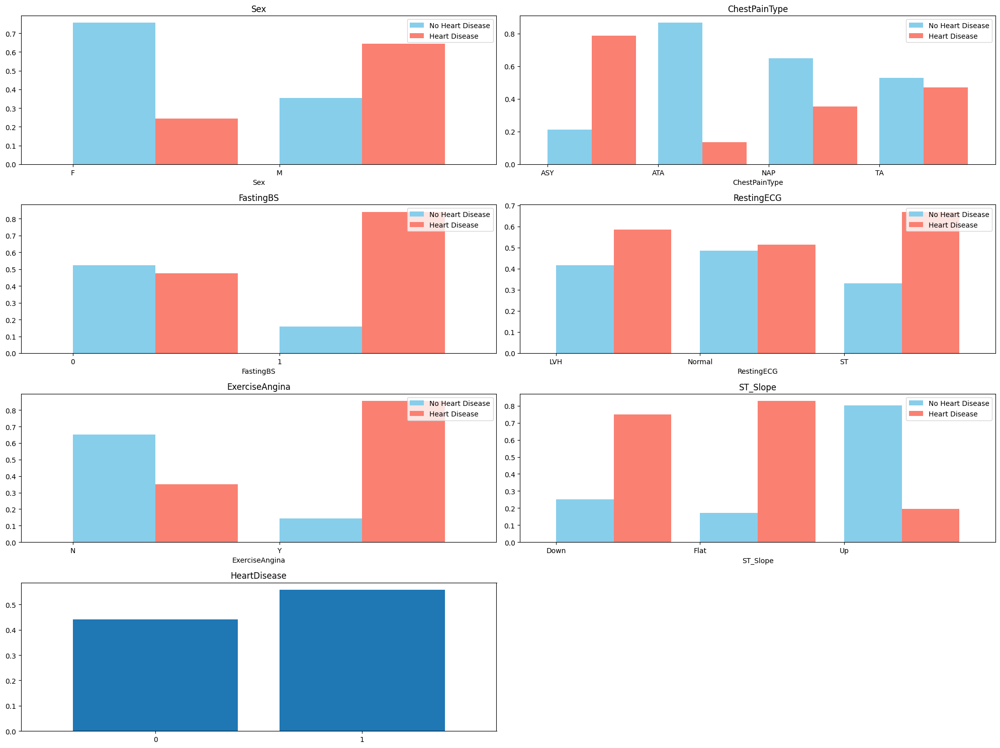
From the plots, we can see that the patients with heart disease have differing proportions in each categorical variable. This suggests that we can include these variables to the logistic regression model.
We also note that there are more males than females in the training dataset. There are also more people with heart disease than not, which raises slight concerns about the representativeness of this dataset.
Multivariate Analysis
We explore the correlation between each numerical predictor variable, using a scatter matrix and correlation heatmap.
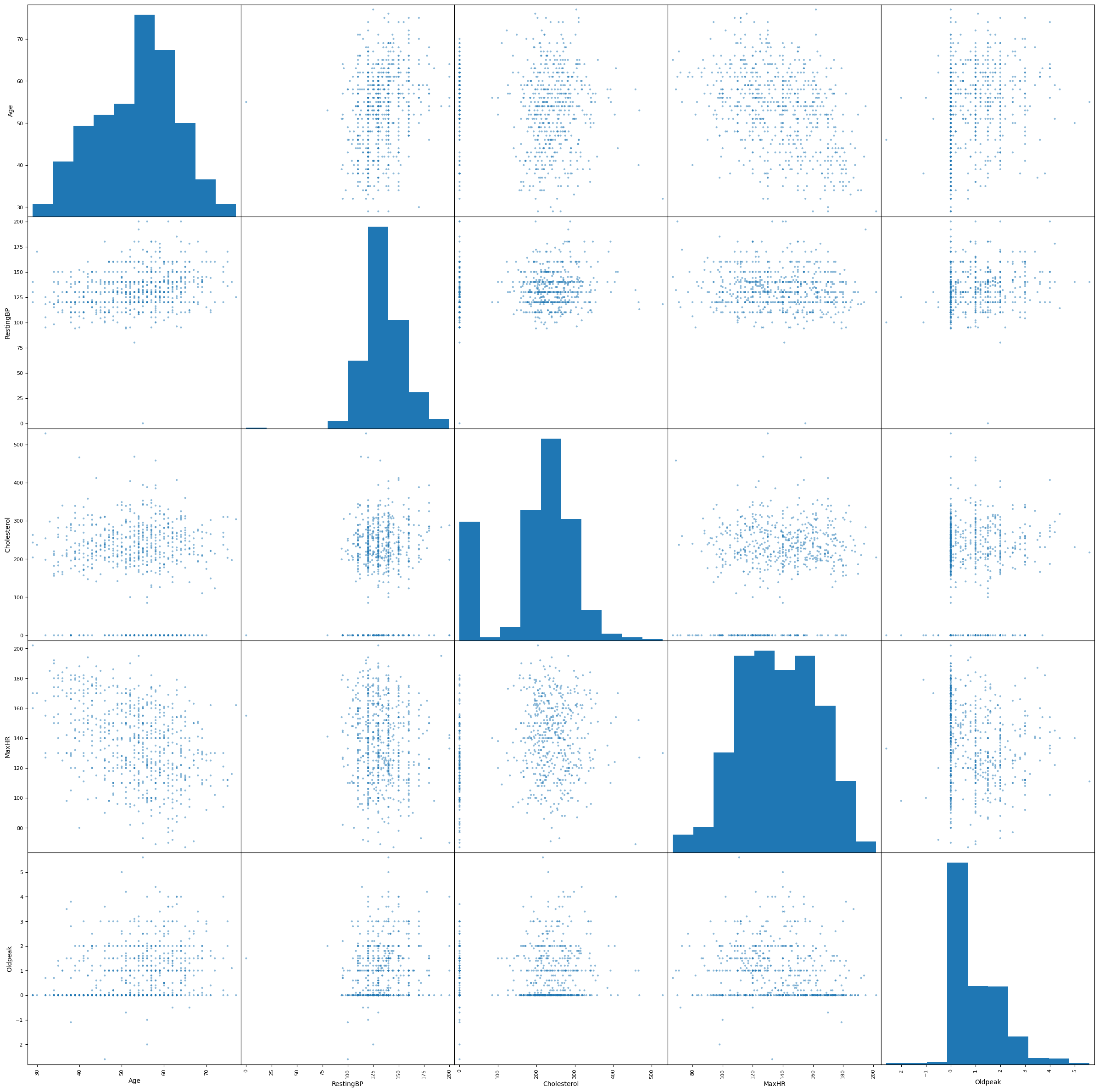
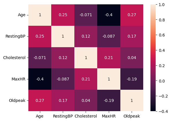
In general, we cannot observe correlation between most ofthe predictors. We may be concerned about the negative correlation between Age and MaxHR.
Next, we check for multicollinearity using Variance Inflation Factors (VIF). We use a cutoff of 10 to determine whether the factor should be removed from our logistic regression model.
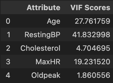
We see that RestingBP has a VIF of nearly 42, so we remove it an check again.
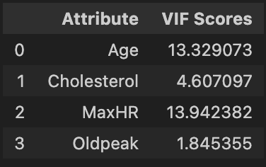
We see that Age and MaxHR both have VIF around 13. We have a choice of which variable to remove, though both are associated with heart disease. We choose to remove MaxHR because of its slightly higher VIF and check for multicollinearity again.

We see that all numerical variables now have VIF under 5. This significant decrease in VIF for Age is in line with our concern of mild correlation between Age and MaxHR.
Finally, we encode for qualitative features before fitting a logistic regression model.
Logistic Regression
Naive Approach
Using the insights from our exploratory data analysis, we will fit a logistic regression model using the 630 observations in the training dataset with Age, Sex, ChestPainType, Cholesterol, FastingBS, RestingECG, ExerciseAngina, Oldpeak, and ST_Slope as predictors. We get a model with the following coefficients:
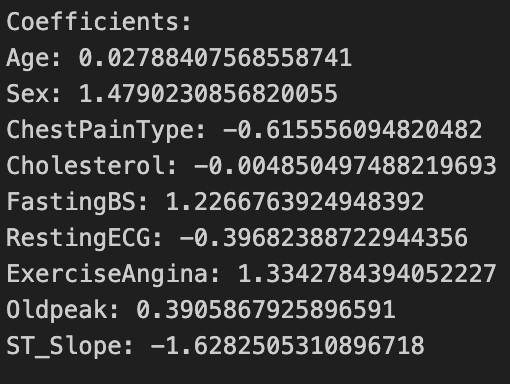
The practical interpretation of these coefficients is different from linear regression. Each coefficient represents the change in the log-odds of heart disease for a one-unit change in the corresponding predictor variable, holding other variables constant. For example, a unit increase in Age leads to a 0.028 increase in the log-odds of heart disease. The prediction accuracy of this model on the testing dataset is 0.8335081.
Alternative Approach I
We stated in the exploratory data analysis that the Cholesterol variable had many observations at 0, which is highly unlikely given the literature. However, it is difficult to remove these observations from the training dataset as we would lose a high proprtion of observations from the training dataset. Moreover, the testing dataset also contains many observations with Cholesterol at 0, so we cannot ignore this problem algother. Finally, we are uncertain about removing the Cholesterol variable given the literature about its link to heart disease.
As such, we utilize two separate logistic regression models to mitigate the effects of these observations. We separate the training and testing data into two groups each: Cholesterol = 0 or Cholesterol > 0.
The first logistic regression model is trained with all observations in the training data, but tested with only testing data with Cholesterol = 0. This model does not use Cholesterol as a predictor. In doing so, we are able to use all observations in the training data to fit a model, mitigating the effect of removing Cholesterol as a predictor.
The second logistic regression model is trained on observations in the training data with Cholesterol > 0 and also tested on observations in the testing data with Cholesterol > 0. This allows us to keep Cholesterol as a predictor in the model for observations that presumably did not have measurement error. The coefficient of Cholesterol in this model was 0.001, which indicates that it is not as strongly associated with heart disease occurance as previously believed.
After merging the predictions of the two models, the prediction accuracy of this model on the testing dataset is 0.83570705, a marginal increase over the previous predictions.
Alternative Approach II
Given that Cholesterol is not strongly associated with heart disease given the other predictors, we try removing Cholesterol as a predictor and fitting a logistic regression model on all observations in the training dataset. This allows us to fit a model with the largest possible number of observations that we have with our data. The prediction accuracy of this model on the testing dataset is 0.8290626.
Alternative Approach III
Finally, we observe that for the observations in the training dataset with Cholesterol = 0 have a 0.89 proportion of having heart disease. Depending on the applications of this model, overdiagnosing heart disease is more beneficial than underdiagnosing. This is especially true when preliminarily diagnosing individuals with heart disease before extensive checks to confirm this.
Thus, we can attempt to map all observations in the testing dataset with Cholesterol = 0 to have heart disease, then fit a logistic regression model on the remaining observations identical to the second model in Alternative Approach I. The prediction accuracy of this model on the testing dataset is 0.84085325, the highest accuracy of all the models so far.
Conclusion
We conducted a thorough exploration of various combinations of observations and predictors to create a predctive model to identify the presence of heart disease. The complexity of selecting the right features and instances underscored the significance of both exploratory data analysis and domain knowledge in ensuring thoughtful data preprocessing and informed feature selection.
a notable limitation surfaced due to the relatively modest sample size in our training and testing datasets. This challenge was further compounded by the presence of problematic observations, either as outliers or values inconsistent with the literature. Recognizing these constraints, it becomes evident that the success of machine learning models is intricately tied to the quality and integrity of the underlying data.
In future studies, it would be beneficial to incorporate additional data sources and try different machine learning models.
References
- Aha, D. W. (n.d.). Heart Disease Data. UCI Machine Learning Repository. Link
- Tada, H., Usui, S., Sakata, K., Takamura, M., & Kawashiri, M. (2020). Low-Density Lipoprotein Cholesterol Level cannot be too Low: Considerations from Clinical Trials, Human Genetics, and Biology. Journal of Atherosclerosis and Thrombosis, 27(6), 489–498. DOI