home..

Stress Analysis

Makoto Takahara / January 2024 (2465 Words, 14 Minutes)

Project Overview

For this project, I worked in a group to investigate the relationship between subjective stress levels and various lifestyle factors.

We used a multiple linear regression to model this relationship with data from Kaggle. This project placed an emphasis on testing the assumptions of linear regression, correcting and mitigating violated assumptions, model selection, and analysis of variance (ANOVA).

---

Project Content

Introduction

This study aims to investigate the association between subjective stress levels and various factors among individuals aged 21 to 35. Our research question focuses on understanding how sleep habits, social interaction levels, meditation, passions, and gender collectively influence the subjective stress experienced by this age group. Employing a multiple linear regression model, we examine lifestyle factors as independent variables and gender as an independent categorical variable, considering literature highlighting its impact on subjective stress (APA, 2012). The linear model evaluates the significance of predictors on stress levels, with positive coefficients for numerical variables indicating increased stress with higher values, and vice versa for negative coefficients. For gender, a positive coefficient implies higher stress for males compared to females, and vice versa for negative coefficients. Statistically significant relationships, determined by p-values below 0.05, are identified, providing a comprehensive and nuanced exploration of how lifestyle factors and gender influence stress levels in individuals aged 21-35.

The existing literature on stress factors offers valuable insights, with Jin’s exploration emphasizing therapeutic activities like meditation and walking, albeit overlooking crucial lifestyle factors such as sleep habits, social interaction, and gender (Jin, 1992). Nollet et al.’s neuroscientific perspective delves into the sleep-stress relationship, but their focus on neurochemistry neglects an examination of sleep’s impact on subjective stress levels (Nollet et al., 2020). In contrast, Cacioppo and Hawkley (2003) touch upon stress within the context of social isolation, yet stress plays a peripheral role in their broader health proxies. Our research model aims to fill this gap by explicitly investigating the association between social interactions and stress, offering a more direct analysis of their relationship. Building upon existing studies, our research addresses the need for a holistic investigation into how a combination of lifestyle factors and individual characteristics collectively influences subjective stress levels.

Methods

Assessing Model Assumptions

Our initial linear regression model takes daily stress as the response variable and a number of lifestyle factors and gender as predictors, presented below:

\[\begin{align*} Daily\ Stress &= \beta_0 + \beta_1 Social\ Network \\ &\quad + \beta_2 Daily\ Steps + \beta_3 Daily\ Sleeping \\ &\quad + \beta_4 Sleep + \beta_5 Screen\ Time\ for\ Passion \\ &\quad + \beta_6 Meditation + \beta_7 Gender + \varepsilon \end{align*}\]

Daily Stress: Likert scale ranging from 1 to 5 (weak to strong)
Social Network: Number of people individuals interact with in a day.
Daily Steps: Number of steps (in thousands) individuals typically walk every day.
Daily Shouting: Number of times individuals shout at somebody in a week.
Sleep: Hours individuals typically sleep.
Time for Passion: Hours individuals spend every day doing what they are passionate about.
Meditation: Number of times individuals think about themselves in a week.
Gender: Categorical variable (1 indicating male and 0 indicating female).

Checking Assumptions of Linear Regression: To assess assumptions in our multiple linear regression analysis, we employ a side-by-side boxplot for gender (categorical) and histograms for lifestyle factor predictors and daily stress. Skewness in response histograms or asymmetry in predictors’ boxplots may indicate violations of linearity or normality assumptions.

Checking Conditions of Multiple Linear Regression: To check the conditional mean response condition, we inspect a “response vs fitted value” scatter plot for daily stress, aiming for a random diagonal scatter to satisfy this condition. The conditional mean predictor condition is assessed through pairwise scatterplots for numerical predictors, meeting the condition if residual plots exhibit no curve or non-linear trend. Violation of these conditions implies that future residual plots cannot pinpoint specific assumption violations.

Checking Assumptions of Linear Regression (Part II): After assessing conditions, we generate residual plots (“residual vs fitted” & “residual vs each predictor”) and a side-by-side boxplot for “Gender.” To check the uncorrelated error assumption, we scan for large clusters in residual plots, as their presence would render the model inappropriate. If absent, we proceed to assess linearity, identifying violations through systematic patterns in residual plots. Box-cox transformations on corresponding predictors follow, involving maximum likelihood estimation for lambda and selecting a simple power. After transforming predictors, we refit the model and reevaluate conditions until linearity improves. Once achieved, we check the normality assumption using a QQ plot, applying box-cox transformations to the response variable as needed. This process repeats until normality is improved. Subsequently, we examine the constant variance assumption by scrutinizing the fanning spread of data points in residual plots. Violations prompt variance stabilizing transformations on the response variable, and we iterate through conditions until constant variance is enhanced.

Model Selection: Ensuring all assumptions are met, we conduct an ANOVA test on the model, evaluating the null hypothesis of no statistically significant linear relationship between all predictors and daily stress. A p-value exceeding 0.05 deems the linear regression model inappropriate; otherwise, further testing is pursued. Individual T-tests are then performed on all predictors, assuming no linear relationship with daily stress. If all p-values are below 0.05, the full model is finalized. Otherwise, predictors with p-values above 0.05 are removed to create a reduced model, followed by a partial F-test. A p-value below 0.05 retains the original full model, while a higher p-value designates the reduced model as final, indicating no significant linear relationship between daily stress and the removed predictors.

Diagnostics

We employ the variance inflation factor (VIF) to assess multicollinearity by calculating VIF values for each predictor. A VIF value below 5 indicates no significant multicollinearity in our model. Should any predictor exhibit a VIF value exceeding 5, we address multicollinearity by removing the predictor with the highest VIF and constructing a reduced model. Subsequently, we reassess the assumptions and conditions for the refined model. To identify potential outliers or influential points, we calculate tool values for each observation, acknowledging values surpassing a predetermined cutoff as limitations in our analysis rather than removing the corresponding observations. This approach aligns with our objective of drawing generalizable conclusions from the model while considering ethical considerations.

Table 1: Tools to Detect Problematic Points and Their Cutoff Values

Problematic Point Type	Measure	Cutoff
Leverage points	Leverage	$> \frac{2(p+1)}{n}$, where $p$ is the number of predictors in our model and $n=6108$ is the total number of observations in our dataset.
Outliers	Standardized residuals of each observation	Not in interval $[-4, 4]$
Observations influential on all fitted values	Cook’s distance	$>$ Median of the F-distribution $F(p+1, n-p-1)$.
Observations influential on their own fitted values	Absolute value of “difference in fitted values” (DFFITS)	$> 2\sqrt{\frac{2(p+1)}{n}}$.
Observations influential on at least one estimated coefficient	Absolute value of “difference in beta” (DFBETAS)	$> \frac{2}{\sqrt{n}}$

Model Selection

After addressing assumptions and handling problematic observations, our model selection is based on the Akaike Information Criterion (AIC) rather than the Bayesian Information Criterion (BIC). AIC strikes a balance between model fit and complexity, proving suitable for scenarios where uncertainty surrounds the true underlying model. We opt for AIC stepwise selection over forward or backward elimination due to its comprehensive approach. This method considers both the addition and removal of variables at each step, capturing complex relationships in the dataset. It iteratively adds or removes predictors based on their impact on the AIC score, ultimately selecting the model with the lowest AIC as the final model.

Results

Data Summary and Description

Table 2.1: Data Summary of Numerical Variables

	Mean	Std. Deviation	Skewness
Sleep	7.11	1.17	-0.29
Meditation	6.09	3.01	-0.13
Social Network	6.17	3.06	-0.01
Time for Passion	3.32	2.71	0.84
Daily Shouting	2.94	2.67	1.11
Daily Steps	5.59	2.91	0.07
Daily Stress	2.81	1.33	-0.07

Table 2.2: Data Summary of Categorical Variable

	Male	Female
Proportion of Gender	42%	58%

Our initial model comprises 7 predictors (Gender + 6 numerical lifestyle factors), with Daily Stress as the response variable, selected from a dataset of 23 variables based on literature and research focus. The chosen predictors—Sleep, Meditation, Social Network, Time for Passion, Daily Shouting, Gender, and Daily Steps—were selected for their conceptual relevance to stress in the literature and context, showing some correlation. Variables excluded were often subjective or lacked literature evidence regarding their association with daily stress. Some were omitted due to vague Likert scale measurements offering only two options.

Model Selection Process

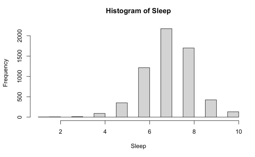
We assessed the skewness of all 7 predictors and the response variable in our initial model. The histogram for Sleep revealed left-skewness, suggesting violated linearity assumption (Figure 1).

Figure 1: Histogram of Sleep

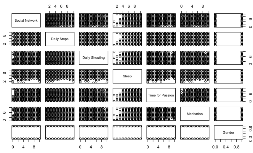
In the multiple linear regression, we first assessed Conditional Mean Response and Conditional Mean Predictor conditions before 4 assumptions. Presented in Figure 2, “Daily stress vs Fitted” scatter plot was checked for a random diagonal scatter pattern, but interpretation was challenging due to Daily Stress being represented as integers on a Likert Scale (1 to 5). Next, we examined residual plots in pairwise scatterplots for all predictors. Despite lacking curvatures, interpretation was challenging due to the predominantly integer nature of the predictors (excluding gender, a categorical variable), and noise in the plots complicated the analysis. Hence, acknowledging uncertainty about meeting additional conditions, we refrained from interpreting residual plots.

Figure 2.1: “Daily stress vs Fitted” scatter plot

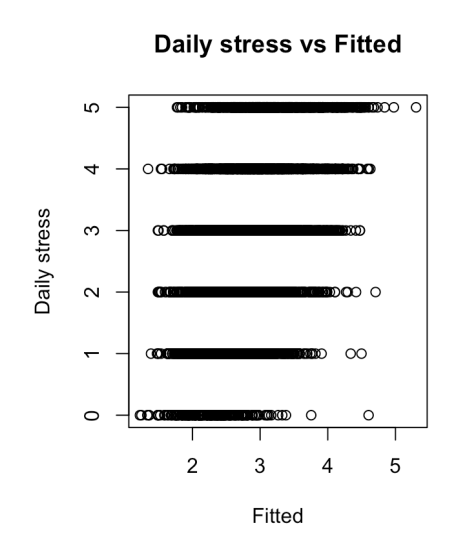
Figure 2.2: Pairwise scatterplots of predictors of initial model

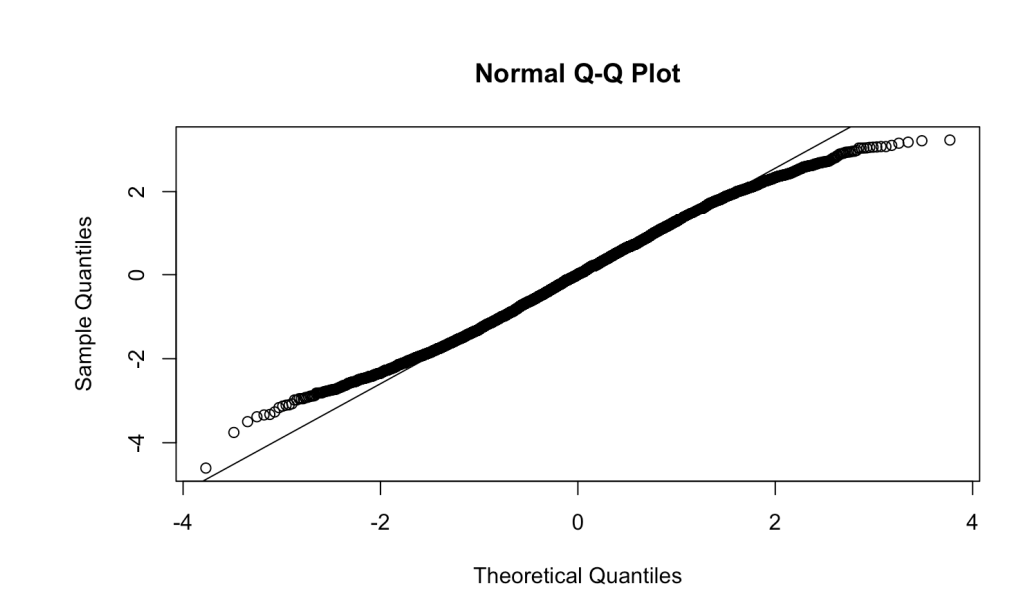
We assessed four assumptions (uncorrelated error, linearity, normality, constant variance) using residual plots for all predictors except gender (a categorical variable), which was evaluated using box plots (Figure 3). Due to the non-interpretable nature of the residual plots, drawing solid conclusions on the four assumptions is challenging. Regarding normality, despite a slight deviation from the diagonal line, considering the integer nature of both the response variable and predictors supports the conclusion that the normality assumption is satisfied. Following our method (written in the previous section), other assumptions also seem to be satisfied based on the assumption plots.

Figure 3.1: Residual plots for initial model

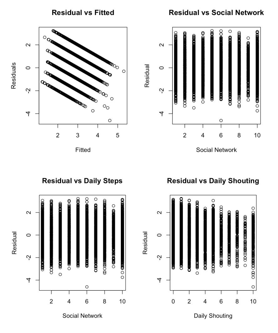
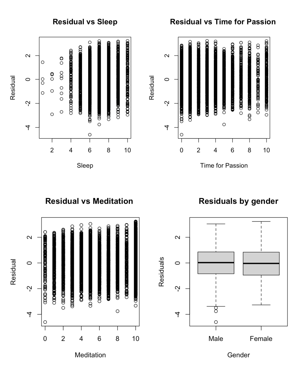
Figure 3.2: QQ-plot for initial model

Addressing the left-skewness of predictor Sleep, a Box-Cox Transformation was applied with a lambda value of 2, creating a new variable squareSleep and replacing Sleep in a new model. Assessment of assumptions for the transformed model revealed similar plots, with squareSleep exhibiting a less skewed histogram compared to Sleep, indicating assumptions satisfaction. An ANOVA F-test confirmed a significant linear relationship between at least one predictor and Daily Stress (p-value < 2.2e^(-16)). Individual T-tests indicated high p-values for Social Network and Daily Steps, leading to their removal in a reduced model. Multicollinearity checks showed all VIF values below 5, indicating no severe issues. Identifying 316 leverage observations (5.1735% of the total) and 299 observations influential on their own fitted values (4.895219% of the total). Additionally, 299 observations were influential on their own fitted values (4.895219% of the total), and over 2429 were influential on at least one estimated coefficient (39.76752%). However, we chose not to remove these observations due to ethical reasons and the potential for biased or incomplete understanding of underlying relationships in the data. The final model includes 5 predictors: Daily Shouting, squareSleep, Time for Passion, Meditation, and Gender.

By AIC stepwise selection, the reduced model from the partial F test, featuring five predictors (Daily Shouting, squareSleep, Time for Passion, Meditation, and Gender), emerged as the most suitable. It holds the lowest AIC value among all considered models, whether incorporating or excluding subsets of the five predictors. This designation as our final model aligns with previous findings. Cross-referencing with alternative methods (forward and backward AIC and BIC), further verified the same optimal model.

Discussion

Conclusion

Initially exploring the impact of lifestyle factors and gender on the subjective stress levels of individuals aged 21 to 35, it culminated in a final model with 5 predictors and corresponding coefficients for our response variable.

\[\begin{align*} Daily\ Stress &= 3.5445 + 0.14057 \times Daily\ Shouting \\ &\quad - 0.00954 \times Square\ Sleep - 0.05521 \times Time\ for\ Passion \\ &\quad - 0.05368 \times Meditation - 0.32961 \times Gender + \varepsilon_i \end{align*}\]

Figure 4 shows the R output for this model.

Figure 4: R Summary of Final Model

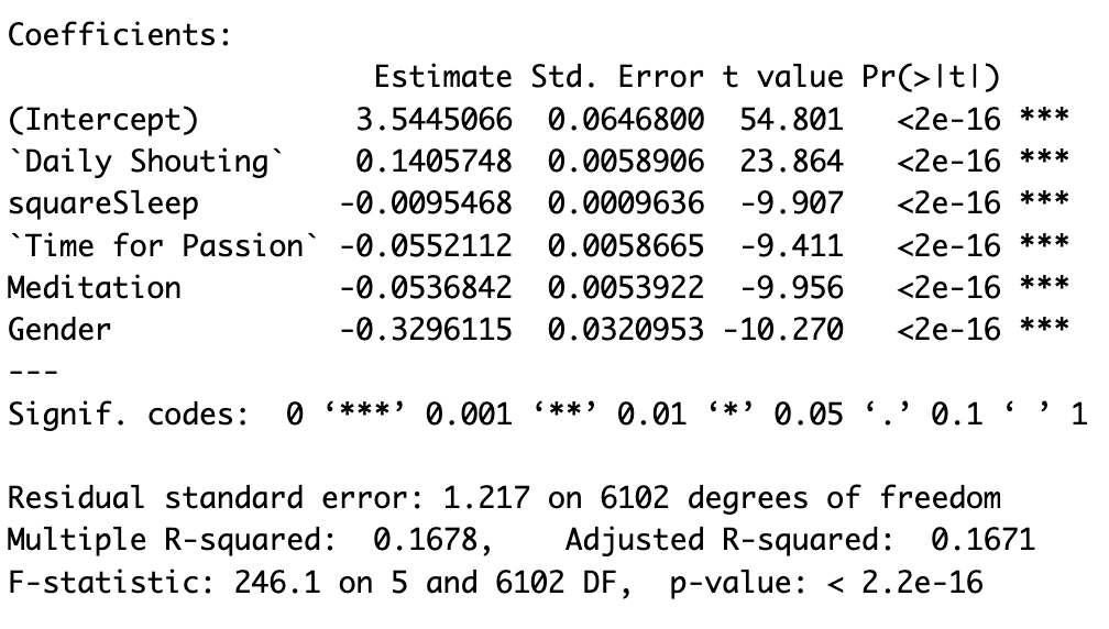
All coefficients demonstrated p-values below 0.05, signifying a significant linear relationship with the response. The model establishes a baseline subjective stress level of 3.5 for female respondents when all lifestyle predictors are at 0. A one-unit increase in Daily Shouting raises average Daily Stress by 0.14 points, while an increase in other non-categorical predictors decreases mean daily stress, assuming fixed values for other predictors. squareSleep is interpreted as a unit increase in the square of Sleep value, leading to a 0.00954 decrease in mean Daily Stress. This aligns with expectations, as sleep, meditation, and time for passions are stress reducers, consistent with literature like Jin (1992) discussing Tai Chi and Meditation’s stress-reducing benefits. Men exhibit lower stress levels than females, indicated by the negative Gender coefficient. While meditation, time for passions, and sleep reduce stress, their impact is significantly smaller compared to shouting, with its coefficient nearly three times greater than the other predictors. In summary, the expected direction of coefficients aligns with literature and initial expectations, but the unexpected magnitude of effects, especially for shouting and gender, was observed. Due to the absence of literature on predictor interactions, we chose not to include interaction terms for model simplicity and to mitigate the risk of false positives.

Limitations

Limitations include potential challenges in satisfying 2 conditions due to the integer nature of variables, introducing residual plot uncertainty. Despite this limitation, we proceeded with the investigation, acknowledging the noise level. Box-Cox transformation resulted in squareSleep replacing Sleep in the model, potentially impacting interpretability. While multicollinearity is a potential limitation, VIF values below 5 mitigate severe impacts on model stability and interpretability. Leverage and influential observations pose another limitation, with the potential to disproportionately influence model parameters. Despite this, ethical concerns led us to retain these observations, avoiding potential bias or incomplete understanding of underlying relationships in the data.

References

1. American Psychological Association. (2012). 2010 gender and stress. American Psychological Association. Link

2. Cacioppo, J. T., & Hawkley, L. C. (2003). Social isolation and health, with an emphasis on underlying mechanisms. Perspectives in Biology and Medicine, 46(3x). DOI

3. Jin, P. (1992). Efficacy of tai chi, brisk walking, meditation, and reading in reducing mental and emotional stress. Journal of Psychosomatic Research, 36(4), 361–370. DOI

4. Nollet, M., Wisden, W., & Franks, N. P. (2020). Sleep deprivation and stress: A reciprocal relationship. Interface Focus, 10(3), 20190092. DOI